What is chart, how to create a chart in excel?

In Microsoft excel a Chart is a built-in tool that allows you to display data in a different chart and graphs formats such as Column, Line, Pie, Bar, Area, X.Y Scatter, Stock, Surface, Doughnut, Bubble and Radar. These charts and graphs help you understand the data in a worksheet by displaying easy analyze from, although we can also see it in sheet but that is a little bit difficult to analyze from the data.

Select the Excel chart or graph format that is best fits your work

Please see the below image Insert >Charts.

how  to create a chart in ms excel

What is Column Chart

Column Chart

A column chart is used to compare value across categories. The Column Chart shows a comparison of one or more series of data points. Such as you can see the monthly sell graph that is showing the difference between month sell. High sell showing the tallest graph and lowest sell showing the lowest graph.

column chart in ms excel

What is Line Chart

line  chart

A line chart is mostly used for showing trends over time. The lines connect each data point so that you can see how the value fluctuating, increased or decreased over a period of month/time.

Such as in the below chart, you can see the graph of monthly sell.

how to make a line graph in excel 2007

Change Chart Type

You can easily change the applied chart type to a different types of charts at any time.

On the Design tab, click Change Chart Type and a new  window displayed from here you can change and  select any other needed chart type.

how to change chart type 

Also Read:

What Is SmartArt In Excel

What is Pie Chart

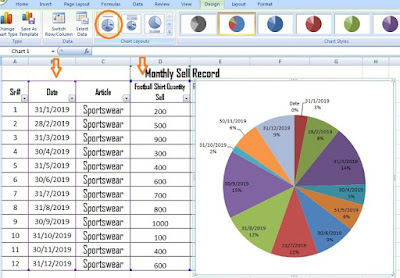
A Pie Chart can only display one series of data. A data series is a row or column of numbers used for charting. Excel uses the first column or row as the chart title.

A pie chart is a circle that divided the data into slices. Each slices represent the contribution in a circle base on its value.

To create a Pie chart on your data sheet select the range and then go to insert >chart use any pie chart subcategory.

You can change the chart name/title. Click on the Chart Title section at the top of the graph and change the title. Now drag anywhere and save it.

If you want to delete the chart place your cursor on the edge of the chart and press your Delete key.

how to add pie chart in excel

Pie  chart with row range

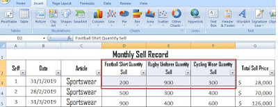
To apply the pie chart on columns first select the column range and choose the pie chart and next to any sub-category.

Pie chart with columns range

What Is Bar Chart

A Bar Chart is a graph that similar to a Column Chart. A bar chart can be used to compare the multiple values in a worksheet. The best uses of the bar chart are when the value on the chart represents duration or when the text is too long.

To make a Bar chart, first we have selected columns B, D, E from our sheet and Click on the Insert tab & then on Bar Chart from the Charts group. You will see many options here when you select this button, such as 2-D, 3-D, cylinder, Cone, Pyramid. For our worksheet, we have selected 2-D columns. The chart will appear. You'll also see horizontal bars giving the names of your headers at the left of your graph.

how to make a bar chart in excel with multiple data

You can change the chart name/title. Click on the Chart Title section at the top of the graph and change the title. Now drag anywhere and save it.

If you want to delete the chart place your cursor on the edge of the chart and press your Delete key.

Further, you can redesign your graphs by using other options. Just go to the Design tab or double click on chart edges it will directly go there. Such as in the below image you can see we have applied next layout 5 from chart layouts.

How to draw a simple bar chart in excel

What is Area Chart

An area chart is similar to a line chart but with one difference. The area below the line in graphs is filled with colours. Area Charts are used primarily to show trends over time or other category.

To apply the Area chart, first select the range and choose the Area chart and next to any sub-category.

How to create an area graph in excel

You will see many options here when you select this button, such as 2-D, 3-D area. For our worksheet, we have selected 3-D Area and next layout 7.

Excel 2007 Area chart

What is smartart in excel?

In Microsoft, excel SmartArt is a function that gives you the ability to quickly and easily create visualize graphical lists, diagrams, and captioned pictures in your worksheet. Smart Art is a way to change simple text into more attractive looks. It can be used to grab attention to important information or make information easier to interpret and understand.

How do you find the SmartArt function in excel?

Go to Excel, click the "Insert" tab. Click the "SmartArt" button  in the Illustrations group on the ribbon below the tab

how to insert SmartArt graphic in excel

 How to choose a SmartArt Graphic

When you click on the Insert>SmartArt a window displayed on your excel screen, select a type of SmartArt graphic on the left menu (All, List, Process, Cycle, Hierarchy, Relationship, Matrix, Pyramid) then select a specific SmartArt subcategory graphic to add to on your worksheet and click OK.. See the below image.

Also Read:

How To Add Shape In Microsoft Excel

How to fill the Text in graphic

To fill the text in the SmartArt graphic, click its [Text] placeholder and then simply type any text. When you finish entering the text in the diagram, click outside the graphic to deselect it.

how to display the choose a SmartArt graphic dialog box

Additional Graphics Option for reshaping or redesign

When you added SmartArt the graphic here you have options to further reshape or redesign it. First, click on SmartArt box and then right-click from the mouse new window display like the below image and use any option on your SmartArt.

Using SmartArt graphic

How to add shapes in Microsoft Excel?

In Microsoft excel there are many different Shape built in which we can use easily in our worksheet according to our work requirement and choice. We can insert readymade shape, such as text box, rectangle, circles, block arrow, line, equation shape flowchart symbol, star and banner, callout, etc.

How to Add Shapes in Microsoft Excel

From the Insert tab, in the Illustrations group, click on Shapes.

Insert shapes tab

To insert a shape simply click on the shape you want from the drop-down menu. Select a shape by clicking on it Excel will automatically choose the default color and style.

Excel custom shapes

When you select any shape, then you can see your cursor will change to a plus sign.

Plus  sign while  adding excel custom shapes

Also Read:

How To Insert Picture In Excel

How to Resize, Rotate and Curve the Shapes

Click in your worksheet where you want to place the shape, and when you added a  shape drag your mouse until the shape is the size you want it to be in a worksheet. 

See the below image for better understanding.

how to resize rotate and curve shape in excel

When shapes inserted in the worksheet you can also use many other options for your shape in the below image you can see options.

Shapes other options in ms excel

How to insert picture in excel cell?

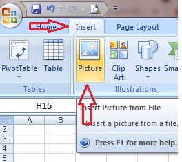
Insert picture option we can use to add images in our worksheet from our computer. To insert images in Excel spreadsheet, go to the Insert tab > Illustrations group, and click the Pictures tab.

how to insert a picture in excel 2007

 In the Insert Picture dialog box that opens, browse to the picture that you want to insert and select it. When picture inserted Resize the picture according to your worksheet requirement.

Browse and insert image in excel worksheet

When image inserted in worksheet here we can see other many options that we can use to redesign our pictures such as in the below images you can see options.

Inserted picture in excel

Please note if the format option not visible on your worksheet double click on inserted images than it will be visible. 

Brightness> We can increase or decrease the brightness of the pictures by using this option.

Contrast> We can increase or decrease the contrast of the pictures.

Recolor> We can use this option to recolor them to give it stylized effects.

Compress Picture>  To reduce the picture size use compress picture.

Change Picture> If want to change picture with different picture use change picture option in this way format, shape, and size remain the same.

Reset Picture> If you want to discard all of the formatting changes you made on the picture use this option.

Picture Style> To change the frame use this option.

Picture shape> change the shape of your picture preserving all the formatting use this option.

  

Picture Border> Use to specify the color, width and line style for the outline of the selected picture shape.

Picture Effects> To apply a visual effect on inserted picture, such  as a shadow, glow, reflection, 3d, and so many others use this option.

Bring to Front> If any specific picture wants to bring in front of all the images so that no part of all the images hidden behind other images use this option. First, select the image and then use this option.

Send to Back> If any specific picture wants to send back of all the images use this option. First, select the image and then use this option.

Selection Pane> Show the selection pane to help select individual objects and to change their order and visibility.

Align> To align the edges of multiple picture, shape of picture use this option. We can also centralized or distribute them evenly across the page. Please note to apply this option first select two or more than two images then align option will be visible.

Group> To merge two or more than two images into a singe treated image use this option.

Rotate> For rotation or flip the image in your worksheet use this option.

Crop> If you want to remove any part of the image use this option.

Height & Width > If you want to change the height & width of image use this option 

Hoodies

What is insert table in excel?

In Ms Excel Insert Table is a function that creates a format on your worksheet to manage and analyze data. Tables make it easy to sort and filter. Excel provides several predefined table styles that we can use rapidly format a table on our worksheet. If built-in table styles don't meet your needs, we can create a custom table style.

Select any cell within the table, or range of cells you want to format as a table.

Go to Insert Tab>Table 

how to create insert table in ms excel 2007

how to insert a table in excel cell

Also Read:
How To Insert Picture In Excel

Further, we can adjust the table formatting by choosing Table Styles options elements, such as Header and Total Rows, First and Last Columns, Banded Rows and Columns, as well as Auto Filtering.

What is pivot table in excel?

In Microsoft Excel, A pivot table is a tool that allows you to review huge quantities of data quickly and easily. With the pivot table, we can build good looking reports for presentation. To understand pivot tables, use it on your worksheet.

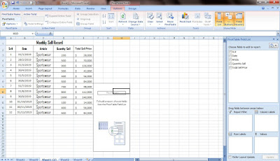
Select your worksheet or just click on any cell and Go to Insert Tab & click on the Pivot table. Excel will display the create Pivot Table window. The default location for a new pivot table is created on a new worksheet. But you can change location according to your work requirements.

pivot table excel example

You can see the pivot table field list is uncheck, now choose/checkmark those fields that you want to add in your reports.

how to create a pivot table in excel

When fields marked your reports will be prepared.

pivot table in excel sales report

Also Read:

How to insert picture in Ms Excel

What is insert table in Microsoft Excel

What is Find and Replace in MS Excel?

In Ms Excel Find & Select is a feature that enables you to quickly find specific text, and replace it with the other text. Especially this is useful when your spreadsheets contain on a large number of data and you need to change certain text on several places repeatedly.

Suppose by mistake you typed a wrong text or value on your worksheet and you want to change it now. Instead of read and typed manually for the correction you just go in Home Find & Replace tab select find and then type wrongly entered data and then replace it with correct word.

Further, you can replace one by one or can use replace all option.

The short cut key for Find & Replace is, > Ctrl+F

find and replace in excel

Please see the below images.

what is find replace and how it works in ms excel

Another option in Find & Replace is you can use Excel's Go To Special feature to quickly find & select all cells which are containing with formulas, comments, conditional formatting, constants, data validation, etc.

Also Read:
What Is Pivot Table In Excel
How To Insert Picture In Excel
oemwes.blogspot.com