What is cell style?

What is cell styles and how to apply?

In Microsoft Excel, a cell style contains different formatting options, which you can quickly apply on your worksheet such as font, sizes & color, comma, percentage, currency formats, cell borders, and shading, etc. You can also modify or duplicate a cell style to create your own, custom cell style. Cell styles are based on the document theme that is applied to the whole workbook. Suppose if you apply currency format it only add dollar sign on number/value.

Please see the below image for better understanding.

Home>Cell Style

how to save cell styles excel

What is Format as table in excel

What is Format as table in excel?

In Excel format as table is a function that quickly formats your worksheet data into a predefined table. Excel provides several predefined table styles which you can use on your worksheet. However, when you apply the predefined table style formula for the selected data, some formatting change applies to your worksheet. If you don't like to work with your data in a table but keep the table style formatting, you can convert the table back to a regular range.

Please see the below image for better understanding.

Home>Format As Table

format as table

Select the data at worksheet and choose an option.

How do format as tables work in Excel

To remove Format as table go to the Design tab Tools group, and click Convert to Range. Or, right-click anywhere within the table, and select Table > Convert to Range.

What is icon set in excel

What is icon set in excel and how do we apply?

In Excel Conditional Formatting Icon Sets mostly used to represent data in a different shape which will make the sheet more significant by using a different kind of shapes.  Icon sets contain various icon formatting shapes like Arrow, Traffic Light, Flag, etc.

To add an icon set, please follow the below steps

Click on conditional formatting > Icon Sets > Select Any Icon.

conditional formatting icon sets the percentage

 By default, for 3 icons, Excel calculates the 67th percent and 33th percent. But you can customize according to your work requirement.  

On status column put again all value or put formula like below screen shoot.

excel 2007 custom icon sets

For customization select the column range and click on Conditional Formatting and select Icon Sets and choose the icon shapes you want to place. After choosing the icon click on More rules.

excel custom icon sets

After click on more rules, we can see various format rules. By default, it works on percent but our work base on value so we have chosen type as a number because the format rule is based on values and not on the percentage which is shown in the below image.

icon set conditional formatting formula

Green Color Flag: if the value is greater than or equal to 200000.

Yellow Color Flag: if the value is less than 200000 and greater than equal to 150000 percent.

Red Color Flag: if the value is less than 150000 percent.

I want to show only icon in status cells, so i marked show only icon but if you unmark it can show value+icon .

Create Your Own Excel Icon Set

What is the colour scale in Excel?

What is the color scale in excel conditional formatting?

In conditional formatting color scales, allocate 3 Color scales to calculate the values in a worksheet. One color fills to represent the lowest value, 2^nd  color represents medium value and 3^rd represents the highest value. This makes it easy to see general patterns in data, especially in large data

Please follow the below images for better understanding.

Click on conditional formatting > Color Scale > Color Option.

excel conditional formatting color scale formula

When the formula applied for datasheet shows like the below image.

How do you use conditional formatting color scales

 

Also, we can change the color scale rules according to our requirement, let’s say we can change color formatting.

After applying the formula click on More rule and customize your own rules according to your work requirements.

excel conditional formatting color scales more rules

What is data bars in excel?

What is data bars and how to add data bars in excel?

In Excel Conditional Formatting Data bars, color scales, are formats that create visual effects in your data. Data bars option can help you mark larger and smaller numbers in color scale. A larger color scale bar represents a larger value, and a small color scale bar represents smaller values.

In short, these conditional formats make it easier to compare the values of a range of cells on a worksheet.

Please follow the below images for better understanding.

Click on conditional formatting > Data Bars > Color Option.

how to add data bars in excel

You can create your own rules to apply on your worksheet by click on More Rule. When you click on more rules here you can see an option and have a right to customization.

how to edit data bars in excel

Excel conditional formatting above and below average

What is the Above/Below Average in Excel Conditional Formatting?

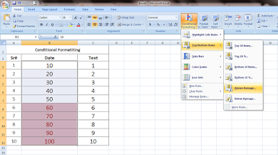
In Excel Conditional Formatting Above Average is a function that quickly highlights those value which averages coming higher from the selected row or column area.

For example, if a spreadsheet contains 10, 20, 30, to 100 value, and when calculating the sum of 10 to 100 answer is 550 and divide it to total figure number which is 10 and the average value comes 55. When we apply the Above Average formula, it highlights those values which are above 55.

Please follow the below images for better understanding.

Click on conditional formatting > Top/Bottom rules > Above Average.

excel conditional formatting above average

Also Read: What Is Color Scale

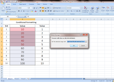
In Excel Conditional Formatting Below Average is a function that quickly highlights those value which averages coming lower from the selected row or column area.

For example, if a spreadsheet contains 10, 20, 30, to 100 value, and when calculating the sum of 10 to 100 answer is 550 and divide it to total figure number which is 10 and the average value comes 55. When we apply the Below Average formula, it highlights those values which are below 55.

excel conditional formatting below average

What is top/bottom ten values in Excel?

What are the top/bottom values and how to change qty to highlight the value in Excel Conditional formatting?

Such as by see the name we can judge the function of this formula.

In Excel Conditional Formatting Top 10 Value is a function that highlight those value which are higher value from the selected row or column area.

For example, if a spreadsheet contain 1 to 100 value, when we apply the top ten value it highlights 90 to 100 value because these are top high values.

Bottom 10 value is another function which highlight the top 10 lower value among the selected row or column area.

For example, if a spreadsheet contain 1 to 100 value, when we apply Bottom ten value it highlights 1 to 10 value because these are the top low value from the selected cells.

how do you find top/bottom ten value in excel

highlight the highest value in excel

By default qty show 10 in right side box but you can change it easily. You can increase or decrease the number of qty by click on up and down small arrow or manually type qty as you need for your work.

In the below image, you can see how to change qty.

how to highlight largest / lowest value in each row

What is the duplicates formula in Excel?

What is duplicates Conditional formatting in Excel?

In Conditional Formatting “Duplicate Value” is a function which highlights those cells' value that contains the same value or text two or more than two times in a row or column. And another function is it can also highlight unique value from the selected cell range.

Please follow the below images for better understanding.

Click on conditional formatting > Highlight cell rules > Duplicate Value.

what is the formula to highlight duplicates value in excel

To highlight duplicate value or any text from the selected cell Click on Duplicate or if you want to highlight a Unique value or text you can choose other Unique options. Kindly note that first select the area from where you want to highlight the values.

excel conditional formatting formula to find duplicate values

What Is Date Occurring In Conditional Formatting?

What Is Date Occurring In Conditional Formatting?

In Conditional Formatting “Date Occurring” is a function which highlights those cells' that contains certain date selected from the given options while applying Date Occurring formula.

Please follow the below images for better understanding.

Click on conditional formatting > Highlight cell rules > Date Occurring.

excel conditional formatting date occurring

Click on Date Occurring a new window open like below image and you can choose any date from the given option according to your work condition.

date occurring conditional formatting in excel

What Is Text That Contain In Conditional Formatting?

What Is Text That Contain In Conditional Formatting?

In Conditional Formatting “Text That Contain” is a function which highlights those cells' or the value that contains certain value or text defined by us while applying Text that contain formulas.

Please follow the below images for better understanding.

Click on conditional formating > Highlight cell rules > Text that Contain.

excel conditional formatting if cell contains specific text

Click on Text That Contains the new window open like below image and you can put value or text such as I want to highlight different text and value.

First I selected the cells from where I want to highlight text and put text ABC & apply formulas.

Second again I want to highlight and put text DEF & apply formulas.

Third again I want to highlight and put a value 101 & apply formulas.

But you can put any value or text that contain in a selected cell according to your work requirement.  

Note: You can use more than one conditional formatting on specific columns, rows or Values at a time.

excel conditional formatting text contains

What Is Equal To In Conditional Formatting?

What Is Equal To In Conditional Formatting?

In Conditional Formatting Equal to function highlight those cells' or value that is certain value define by us while applying Equal to formulas.

.

Please follow the below images for better understanding.

Click on conditional formating > Highlight cell rules > Equal to.

what is equal to in conditional formatting

By click on Equal to the new window open like below image and you could put value such as I want to highlight (Green Fill With Dark Green Text) those values which are equal to 50 among the cells. 

Note: You can use more than one conditional formatting on specific columns, rows or Values at a time.

how to do conditional formatting equal to in excel

What is Between in Conditional Formatting?

What is Between in Conditional Formatting?

In Conditional Formatting Between function highlight those cells' or value that is "greater than and less than ", certain value define by us while applying between formulas.

You can use a simple formula that returns TRUE when the value meets those conditions.

Please follow the below images for better understanding.

Click on conditional formating > Highlight cell rules > Between.

By click on Between new window open like below image and you could put value such as I want to highlight (Green Fill With Dark Green Text) those values which are Greater Than 25 and Less than 60 from the cells. 

Note: You can use more than one conditional formatting on specific columns, rows or Values at a time.  

excel conditional formatting formula greater than and less than

What is Less Than Conditional Formatting?

What is Less Than Conditional Formatting?

In Conditional Formatting Less than feature highlight those cells' or value that is Less than a certain number define by us while applying Less than tools.

Please follow the below pictures.

Click on conditional formating > Highlight cell rules > Less Than rules.

excel conditional formatting formula less than

By click on Less Than Rules new window open like below image and you could put value such as I want to highlight (Yellow Fill With Dark Yellow Text) those values which are Less than 45 from the cells. 
Note: You can use more than one conditional formatting on specific columns, rows or Values.  

What Is Conditional Formatting?

What Is Conditional Formatting?

Conditional formatting in MS Excel is a very interesting, useful and time saving command.

For example, if you have a spreadsheet with thousands of rows or columns of data. It would be extremely difficult to see or search specific data from thousands of rows or cells. MS Excel gives us several tools option that will make this task easier. With conditional formatting, we can apply formatting to one or thousand cells based on the value of the cell. You can highlight any specific value and visualize the data using formatting such as data bars.

What is Greater Than Conditional Formatting?

In Conditional Formatting greater than feature highlight the those cells' value that is greater than a certain number define by us while applying greater than tools.

Please follow the below pictures.

Click on conditional formating > Highlight cell rules > Greater Than rules.

how do you apply conditional formatting in excel

By click on Greater Than Rules new window open like below image and you could put value such as I want to highlight (Light Red Fill With Dark Red Text) those values which are greater than 25 from the cells.

how do i use conditional formatting greater than in excel

What Is Cut, Copy, Paste, and Paste Special in Microsoft Excel?

What Is Cut, Copy, Paste and Paste Special in MS Excel?

Cut, Copy, Paste, and Format Painter are default built in a format in Microsoft Excel.

How To Cut Or Copy and paste?

For Cut Select the cell which you want to cut and click the cut command on the home tab or use your keyboard button and press CTRL+X. 

For Copy Select the cell which you want to copy and click the copy command on the home tab or use your keyboard button and press CTRL+C.

For Paste Select the other cell where you want to paste your text and click paste command from the home tab or use your keyboard button and press CTRL+V. 

how to cut copy and paste in excel

Paste Special is a menu option. If you want to paste only a specific aspect of the copied data like its value, formulas, formatting, comments, etc you would use one of the Paste Special options after copy or cut data by press Ctrl+Alt+V, or Alt+E+S or command on home tab paste>paste special or right click on a cell where you put data and click paste special option to open the Paste Special menu bar and choose your desired option.

how to paste special values in excel

how to copy paste special values in excel

What is the Format Painter in Microsoft Excel?

What is the Format Painter in Microsoft Excel?

Format Painter is a function in MS Excel that is used when you want to copy only formatting from one cell to another. For example, if you have written text in a cell and it has using a specific font type, color, and font size, borders etc, you could copy that formatting to another cell of text by using the Format Painter tool option. See the below image for understanding.

what is format painter in excel

How to increase or decrease decimal in MS Excel?

How to increase or decrease decimal in MS Excel?

The Increase Decimal and Decrease Decimal are default button setting in MS Excel.

  

If you want to increase decimal on a number Click the Increase Decimal or if you want to decrease Decimal click on decrease decimal button. Each click adds or removes a decimal.

Please see the below image for better understanding.

how to increase or decrease decimal in excel 

What is Comma Format Style In Microsoft Excel?

What is Comma Format Style In Microsoft Excel?

Demonstrate the value of the cell with a thousand separators and you can easily understand the values.

Comma Style format also famous as the thousands separator in MS Excel.  Comma format inserts commas in larger numbers to separate a hundred, thousand, millions, billions and adds two decimals with the values (for example 5000 be converted into 5,000.00). And present negative values in closed parentheses.
 

What is comma style format in MS excel

What is the Percentage ( % ) Symbol In MS Excel?

What is the Percentage ( % ) Symbol In MS Excel?

When you select a cell that already contains numbers and click on % Percentage format Excel multiplies those numbers by 100 and adds the percent (%) sign at the end such as you can see in the below picture. How to apply percentage and what result may come. 

What is the percentage number format in MS excel