What is Microsoft(MS) Excel?
Microsoft Excel is a software program created by Microsoft that allows users to regulate, design and calculate data with formulas using a spreadsheet system.
Normally it use in Office work, organization, an institute that's extremely valuable for many businesses, which use it to record expenditures and revenue, plan budgets, chart data but we can also use it for our personal wok.
We can manage our work by entering data and keep it safe for long term record as we needed.
 |
| Microsoft Excel Work Sheet |
Is Microsoft Excel important?
Yes, it is so important. Among the computer programs which exist, Microsoft Excel is one of the most important because of the key role it plays in many sectors. Many businesses, personal and institutional enterprises have embraced the use of Excel because of its utility and the ability to serve as a visual basic for different applications
What are the benefits of Microsoft Excel?
It is easy to use not any complication for simple work.
It is easy to store the data.
Easy to add or remove rows and columns.
Formulas make it more applicable for business, institute, individual and other works.
Make an easy template design according to our work conditions.
Filter, access and highlight our require data.
How would you start MS Excel?
Just install MS Office Excel from CD/DVD or you can also download and install from the online source.
Open Excel Starter with the Windows Start button.
- Click the Start button. If Excel Starter is not included among the list of programs you see, click All Programs, and then click Microsoft Office Starter.
Click the Microsoft Excel folder and you will see Microsoft Office Excel file, click right click on this icon and other window displays send to and then desktop creates a short cut.
 |
| how to open ms excel in computer |
How to use Microsoft Excel?
When you installed Ms office Excel create a short cut on your desktop, it will show you like the below picture.
| excel icon on desktop |
Double click on excel short cut icon and it will open like below picture and now you can make your desired style format for your work. You can make a daily, monthly, yearly record by using the option provided by Microsoft Office.
What are Rows and Columns in Microsoft Excel?
In MS Excel Row numbers range from 1 to 1048576; in total 1048576 rows and Columns range from A to XFD; in total 16384 columns.
A column is a vertical series of cells in the sheet. Above letters A, B, C, D, to XFD are the column of Microsoft Excel in a spreadsheet. As you can see in the below image.
The Row is a horizontal series of cells in a spreadsheet. The row is placed to the left side of the column containing the numbers 1, 2, 3 and so on.
Please see the below image for a better understanding.
 |
| what are rows and columns in excel |
What is the Home tab in Microsoft Excel?
In Microsoft Office Excel, the Home tab is the default tab in Microsoft Excel The Home tab allows you to change document settings.
Home Tab contains most common and frequently used commands such as cut copy paste underlined bold, text font, text size, text and columns color option, conditional formatting, formula's, etc.
Home Tab contains most common and frequently used commands such as cut copy paste underlined bold, text font, text size, text and columns color option, conditional formatting, formula's, etc.
How To Change Font In Excel?
Home Change Fonts you can type any text here by using your keyboard buttons. You can also change font for your text. Select your text which you want to change then click on downward small icon and select your desired font.

how to change font style in ms excel

How To Resize Text In MS Excel?
Home Resize Text To change the size of the font in a cell or range of cells in a worksheet, click this button. Move the mouse pointer over each of the sizes to see a Live Preview. A list of different font sizes will appear. We can also resize by clicking A one option increase and one option decrease the text size. |
| How to resize text in MS Excel |
How Text Bold/Italic/Underline/Colour Cell Or Colour Text In MS Excel?
Home Text Bold/Italic/Underline/Colour Cell/Color Text To apply bold formattingTo apply bold formatting text in a cell or range of cells, click this button B.
To change the general style of the font into italics, click this button I.
To change the general text style into underline the text in a cell or range of cells clicks this button U.
To change the general text color in any custom colour click on this button A underline with color.
To change the cell or row color into another color click right side icon A underline with color.
By click on this option such as you can see in the below picture, you can change your work according to your desired/required format.
 |
| How to bold, italic, underline, color text in MS Excel |
How To Border Text In MS Excel?
Home Border In the Microsoft Excel program, borders is a gadget that users right to use to add a border around two
or more cells on a spreadsheet. You can use custom design borders such as Bottom
border, Top border, Right border, Left Border, No border, All border, Outside
border, Thick border, etc. You can also use draw your own desire border
by using draw border tool. You can change border colors and design.
 |
| How to border cells in MS excel |
How To Text Align In MS Excel?
Home Text Alignment Select cell or range of cells. Click either the Left Align, Right Align, Center, Middle Align or Top Align, Bottom Align, buttons on the Standard toolbar. The text aligned when you select your desired option and you can see a live preview.
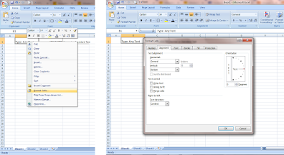
The second option for rotation is to Select the cell(s) that you wish to rotate the text Right click and then select (Format Cells) from the popup menu. When the Format Cells window appears, select the Alignment tab. Then set the number of degrees that you wish to rotate the text.
 |
| how to align text in excel cell |
How To Text Rotate In MS Excel?
Text Rotation You can rotate text in MS Excel to a diagonal angel or vertical orientation. You can click option display on the tab and select your desired rotation option. By chosing the rotation option it works display you as below picture. |
| how to rotate text in excel |
The second option for rotation is to Select the cell(s) that you wish to rotate the text Right click and then select (Format Cells) from the popup menu. When the Format Cells window appears, select the Alignment tab. Then set the number of degrees that you wish to rotate the text.
How To Increase Or Decrease Margin Between the Border & Text?
To increase or decrease margins between the border ad text in Microsoft we have a default built-in format which we can use
We can use the below option to increase or decrease the margin between the border and text. With this option also we can use the space button and backspace button to increase or decrease the margin between text and border.
We can use the below option to increase or decrease the margin between the border and text. With this option also we can use the space button and backspace button to increase or decrease the margin between text and border.
 |
| how to set margin between border and text in ms excel |
What Is Wrap Text In MS Excel?
In Microsoft Excel, Wrap Text is a function that makes you able to adjust your long text in a cell. Wrap text can also be used if any text that goes to the next line without pressing the Enter key.
 |
| What is wrap text in ms excel |
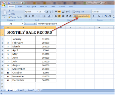
What is Merge and Centre in MS Excel?
In MS-Excel Merging & Center is a default function that
allows you to merge/join two or more different cells in a spreadsheet vertically or horizontally into one larger cell. when data is inserted to
any cell and merged & Center function applies on requiredcells it centralized the position of the text. If you want unmerge then, reclicking on
the merge & center button unmerge the cells but the value
in the cell merged is placed to
the initial first.
 |
| what is merge and center in ms excel |
What is the General Option in MS Excel?
General Option in Excel is a default number format that applies when you type a number. You can use default option how the values display in a cell as a general number, date, time currency, percentage, fraction, Scientific or text.
 |
| what is general number format in excel |
Other option to open General window format just right-click on mouse and a window displayed here an option with format cell and click on this other window will be displayed, in first tab General option open and you can use option according to your work condition.
 |
| What is the general number format in excel |
What Is Accounting Number Format or Currency Symbols in MS Excel?
Accounting
Number Format is a default
currency symbol. By selecting the cell or range of cells, and then clicking Accounting Number Format and select any
currency symbol which you want to display with number/amount.
The standard accounting format contains two
decimal points, a thousand separator, and locks the dollar sign to the far
left side of the cell. Negative numbers are displayed in parentheses.
 |
| what is accounting number format in excel |
Here Five option which we can use for $ symbol on any number.
- 1- Accounting Number Format Or $ Symbol
- 2- In General (Currency) Option
- 3- In General (Accounting) Option
- 4- By Press CTRL+SHIFT+$
- 5- By Edit and Put $ With Keyboard Button
The Accounting format aligns the
dollar signs at the left edge of the cell and
displayed a . for zero values. Negative
numbers are displayed in parentheses.
In General, the Currency format places the
dollar sign right next to the number and displayed
a . for zero values. The Currency format displayed negative
numbers with a minus (-) sign.
In General, the Accounting format aligns the
dollar signs at the left edge of the cell and
displayed a . for zero values. Negative
numbers are displayed in parentheses.
Press CTRL+SHIFT+$ places
the dollar sign right next to the number and displayed
a . for zero values. It displayed negative numbers with parentheses but
in red.
By Edit and Put $ With
Keyboard Button places the dollar sign right next to the number. It displayed
negative numbers with parentheses but in red.
 |
| How to add currency in MS excel |
What is the Percentage ( % ) Symbol In MS Excel?
When you select a cell that already contains numbers and click on % Percentage format Excel multiplies those numbers by 100 and add the percent (%) sign at the end such as you can see in the below picture. How to apply percentage and what result may come.
 |
| What is the percentage number format in MS excel |
What is Comma Format Style In Microsoft Excel?
Demonstrate the value of
cell with a thousand separators and you can easily understand the values.
Comma Style
format also famous as the thousands separator in MS Excel. Comma format inserts commas in larger
numbers to separate a hundred, thousand, millions, billions and adds two decimals with
the values (for example 5000 be converted into 5,000.00). And present negative
values in closed parentheses.
 |
| What is comma style format in MS excel |
How to increase or decrease decimal in MS Excel?
The Increase Decimal and Decrease Decimal are default button setting in MS Excel.
If you want to increase decimal on a number Click the Increase Decimal or if you want to decrease Decimal click on decrease decimal button. Each click adds or removes a decimal.
Please see the below image for better understanding.
 |
| how to increase or decrease decimal in excel |
What Is Cut, Copy, Paste and Paste Special in MS Excel?
Cut, Copy, Paste, and Format Painter are default built in a format in Microsoft Excel.How To Cut Or Copy and paste?
For Cut Select the cell which you want to cut and click the cut command on the home tab or use your keyboard button and press CTRL+X.
For Copy Select the cell which you want to copy and click the copy command on the home tab or use your keyboard button and press CTRL+C.
 |
| how to paste special values in excel |
 |
| how to copy paste special values in excel |
What is the Format Painter in Microsoft Excel?
Format Painter is a function in MS Excel that is used when you want to copy only formatting from one cell to another. For example, if you have written text in a cell and it has using a specific font type, color, and font size, borders etc, you could copy that formatting to another cell of text by using the Format Painter tool option. See the below image for understanding.

what is format painter in excel
 |
| what is format painter in excel |
What Is Conditional Formatting?
Conditional formatting in MS Excel is a very interesting, useful and time saving command.
For example, if you have a spreadsheet with thousands of rows or columns of data. It would be extremely difficult to see or search specific data from thousands of rows or cells. MS Excel gives us several tools option that will make this task easier. With conditional formatting, we can apply formatting to one or thousand cells based on the value of the cell. You can highlight any specific value and visualize the data using formatting such as data bars.
What is Greater Than Conditional Formatting?
In Conditional Formatting greater than feature highlight the those cells' value that is greater than a certain number define by us while applying greater than tools.
Please follow the below pictures.
Click on conditional formating > Highlight cell rules > Greater Than rules.
Please follow the below pictures.
 |
| how do you apply conditional formatting in excel |
By click on Greater Than Rules new window open like below image and you could put value such as I want to highlight (Light Red Fill With Dark Red Text) those values which are greater than 25 from the cells.
 |
| how do i use conditional formatting greater than in excel |
What is Less Than Conditional Formatting?
In Conditional Formatting Less than feature highlight those cells' or value that is Less than a certain number define by us while applying Less than tools.
Please follow the below pictures.
Click on conditional formating > Highlight cell rules > Less Than rules.
By click on Less Than Rules new window open like below image and you could put value such as I want to highlight (Yellow Fill With Dark Yellow Text) those values which are Less than 45 from the cells.
Note: You can use more than one conditional formatting on specific columns, rows or Values.

what is less than conditional formatting in excel
What is Between in Conditional Formatting?
In Conditional Formatting Between function highlight those cells' or value that is "greater than and less than ", certain value define by us while applying between formulas.
You can use a simple formula that returns TRUE when the value meets those conditions.
Please follow the below images for better understanding.
Click on conditional formating > Highlight cell rules > Between.
By click on Between new window open like below image and you could put value such as I want to highlight (Green Fill With Dark Green Text) those values which are Greater Than 25 and Less than 60 from the cells.
Note: You can use more than one conditional formatting on specific columns, rows or Values at a time.

excel conditional formatting formula greater than and less than
What Is Equal To In Conditional Formatting?
In Conditional Formatting Equal to function highlight those cells' or value that is certain value define by us while applying Equal to formulas.
.
Please follow the below images for better understanding.
Click on conditional formating > Highlight cell rules > Equal to.

what is equal to in conditional formatting
By click on Equal to the new window open like below image and you could put value such as I want to highlight (Green Fill With Dark Green Text) those values which are equal to 50 among the cells.
Note: You can use more than one conditional formatting on specific columns, rows or Values at a time.

how to do conditional formatting equal to in excel
In Conditional Formatting Less than feature highlight those cells' or value that is Less than a certain number define by us while applying Less than tools.
Please follow the below pictures.
Click on conditional formating > Highlight cell rules > Less Than rules.
By click on Less Than Rules new window open like below image and you could put value such as I want to highlight (Yellow Fill With Dark Yellow Text) those values which are Less than 45 from the cells.
Note: You can use more than one conditional formatting on specific columns, rows or Values.
Note: You can use more than one conditional formatting on specific columns, rows or Values.
 |
| what is less than conditional formatting in excel |
What is Between in Conditional Formatting?
In Conditional Formatting Between function highlight those cells' or value that is "greater than and less than ", certain value define by us while applying between formulas.
You can use a simple formula that returns TRUE when the value meets those conditions.
Please follow the below images for better understanding.
Click on conditional formating > Highlight cell rules > Between.
By click on Between new window open like below image and you could put value such as I want to highlight (Green Fill With Dark Green Text) those values which are Greater Than 25 and Less than 60 from the cells.
Note: You can use more than one conditional formatting on specific columns, rows or Values at a time.
 |
| excel conditional formatting formula greater than and less than |
What Is Equal To In Conditional Formatting?
In Conditional Formatting Equal to function highlight those cells' or value that is certain value define by us while applying Equal to formulas.
.
Please follow the below images for better understanding.
Click on conditional formating > Highlight cell rules > Equal to.
 |
| what is equal to in conditional formatting |
By click on Equal to the new window open like below image and you could put value such as I want to highlight (Green Fill With Dark Green Text) those values which are equal to 50 among the cells.
Note: You can use more than one conditional formatting on specific columns, rows or Values at a time.
 |
| how to do conditional formatting equal to in excel |
What Is Text That Contain In Conditional Formatting?
In Conditional Formatting “Text That Contain” is a function which highlights those cells' or the value that contains certain value or text defined by us while applying Text that contain formulas.

excel conditional formatting if cell contains specific text
Click on Text That Contains the new window open like below image and you can put value or text such as I want to highlight different text and value.
First I selected the cells from where I want to highlight text and put text ABC & apply formulas.
But you can put any value or text that contain in a selected cell according to your work requirement.
Note: You can use more than one conditional formatting on specific columns, rows or Values at a time.
excel conditional formatting text contains
What Is Date Occurring In Conditional Formatting?
In Conditional Formatting “Date Occurring” is a function which highlights those cells' that contains certain date selected from the given options while applying Date Occurring formula.

excel conditional formatting date occurring
Click on Date Occurring a new window open like below image and you can choose any date from the given option according to your work condition.

date occurring conditional formatting in excel
In Conditional Formatting “Text That Contain” is a function which highlights those cells' or the value that contains certain value or text defined by us while applying Text that contain formulas.
Click on conditional formating > Highlight cell rules > Text that Contain.
 |
| excel conditional formatting if cell contains specific text |
Click on Text That Contains the new window open like below image and you can put value or text such as I want to highlight different text and value.
First I selected the cells from where I want to highlight text and put text ABC & apply formulas.
Second again I want to highlight and put text DEF & apply formulas.
Third again I want to highlight and put a value 101 & apply formulas.
But you can put any value or text that contain in a selected cell according to your work requirement.
Note: You can use more than one conditional formatting on specific columns, rows or Values at a time.
excel conditional formatting text contains
|
What Is Date Occurring In Conditional Formatting?
In Conditional Formatting “Date Occurring” is a function which highlights those cells' that contains certain date selected from the given options while applying Date Occurring formula.
 |
| excel conditional formatting date occurring |
Click on Date Occurring a new window open like below image and you can choose any date from the given option according to your work condition.
 |
| date occurring conditional formatting in excel |
What is duplicates Conditional formatting in Excel?
In Conditional Formatting “Duplicate Value” is a function which highlights those cells' value that contains the same value or text two or more than two times in a row or column. And another function is it can also highlight unique value from the selected cell range.
Please follow the below images for better understanding.

what is the formula to highlight duplicates value in excel
To highlight duplicate value or any text from the selected cell Click on Duplicate or if you want to highlight a Unique value or text you can choose other Unique options. Kindly note that first select the area from where you want to highlight the values.
excel conditional formatting formula to find duplicate values
In Conditional Formatting “Duplicate Value” is a function which highlights those cells' value that contains the same value or text two or more than two times in a row or column. And another function is it can also highlight unique value from the selected cell range.
Please follow the below images for better understanding.
 |
| what is the formula to highlight duplicates value in excel |
To highlight duplicate value or any text from the selected cell Click on Duplicate or if you want to highlight a Unique value or text you can choose other Unique options. Kindly note that first select the area from where you want to highlight the values.
excel conditional formatting formula to find duplicate values
|
What are the top/bottom values and how to change qty to highlight the value in Excel Conditional formatting?
Such as by see the name we can judge the function of this formula.
In Excel Conditional Formatting Top 10 Value is a function that highlights those values which is a higher value from the selected row or column area.
For example, if a spreadsheet contains 1 to 100 value, when we apply the top ten value it highlights 90 to 100 value because these are top high values.
The bottom 10 value is another function that highlights the top 10 lower value among the selected row or column area.
For example, if a spreadsheet contains 1 to 100 value, when we apply Bottom ten value it highlights 1 to 10 value because these are the top low value from the selected cells.

how do you find top/bottom ten value in excel

highlight the highest value in excel
By default qty show 10 in right side box but you can change it easily. You can increase or decrease the number of qty by click on up and down small arrow or manually type qty as you need for your work.
What is the Above/Below Average in Excel Conditional Formatting?
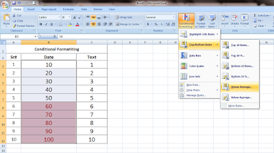
In Excel Conditional Formatting Above Average is a function that quickly highlights those value which averages coming higher from the selected row or column area.
For example, if a spreadsheet contains 10, 20, 30, to 100 value, and when calculating the sum of 10 to 100 answer is 550 and divide it to total figure number which is 10 and the average value comes 55. When we apply the Above Average formula, it highlights those values which are above 55.
Please follow the below images for better understanding.
excel conditional formatting above average
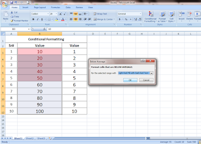
In Excel Conditional Formatting Below Average is a function that quickly highlights those value which averages coming lower from the selected row or column area.
For example, if a spreadsheet contains 10, 20, 30, to 100 value, and when calculating the sum of 10 to 100 answer is 550 and divide it to total figure number which is 10 and the average value comes 55. When we apply the Below Average formula, it highlights those values which are below 55.
excel conditional formatting below average
What is the Above/Below Average in Excel Conditional Formatting?
In Excel Conditional Formatting Above Average is a function that quickly highlights those value which averages coming higher from the selected row or column area.
For example, if a spreadsheet contains 10, 20, 30, to 100 value, and when calculating the sum of 10 to 100 answer is 550 and divide it to total figure number which is 10 and the average value comes 55. When we apply the Above Average formula, it highlights those values which are above 55.
Please follow the below images for better understanding.

excel conditional formatting above average
In Excel Conditional Formatting Below Average is a function that quickly highlights those value which averages coming lower from the selected row or column area.
For example, if a spreadsheet contains 10, 20, 30, to 100 value, and when calculating the sum of 10 to 100 answer is 550 and divide it to total figure number which is 10 and the average value comes 55. When we apply the Below Average formula, it highlights those values which are below 55.

excel conditional formatting below average
Such as by see the name we can judge the function of this formula.
In Excel Conditional Formatting Top 10 Value is a function that highlights those values which is a higher value from the selected row or column area.
For example, if a spreadsheet contains 1 to 100 value, when we apply the top ten value it highlights 90 to 100 value because these are top high values.
The bottom 10 value is another function that highlights the top 10 lower value among the selected row or column area.
 |
| how do you find top/bottom ten value in excel |
 |
| highlight the highest value in excel |
By default qty show 10 in right side box but you can change it easily. You can increase or decrease the number of qty by click on up and down small arrow or manually type qty as you need for your work.
What is the Above/Below Average in Excel Conditional Formatting?
In Excel Conditional Formatting Above Average is a function that quickly highlights those value which averages coming higher from the selected row or column area.
For example, if a spreadsheet contains 10, 20, 30, to 100 value, and when calculating the sum of 10 to 100 answer is 550 and divide it to total figure number which is 10 and the average value comes 55. When we apply the Above Average formula, it highlights those values which are above 55.
Please follow the below images for better understanding.
 |
| excel conditional formatting above average |
In Excel Conditional Formatting Below Average is a function that quickly highlights those value which averages coming lower from the selected row or column area.
For example, if a spreadsheet contains 10, 20, 30, to 100 value, and when calculating the sum of 10 to 100 answer is 550 and divide it to total figure number which is 10 and the average value comes 55. When we apply the Below Average formula, it highlights those values which are below 55.
 |
| excel conditional formatting below average |
What is the Above/Below Average in Excel Conditional Formatting?
In Excel Conditional Formatting Above Average is a function that quickly highlights those value which averages coming higher from the selected row or column area.
For example, if a spreadsheet contains 10, 20, 30, to 100 value, and when calculating the sum of 10 to 100 answer is 550 and divide it to total figure number which is 10 and the average value comes 55. When we apply the Above Average formula, it highlights those values which are above 55.
Please follow the below images for better understanding.
 |
| excel conditional formatting above average |
In Excel Conditional Formatting Below Average is a function that quickly highlights those value which averages coming lower from the selected row or column area.
For example, if a spreadsheet contains 10, 20, 30, to 100 value, and when calculating the sum of 10 to 100 answer is 550 and divide it to total figure number which is 10 and the average value comes 55. When we apply the Below Average formula, it highlights those values which are below 55.
 |
| excel conditional formatting below average |
What is data bars and how to add data bars in excel?
In Excel Conditional Formatting Data bars, color scales, are formats that create visual effects in your data. Data bars option can help you mark larger and smaller numbers in color scale. A larger color scale bar represents a larger value, and a small color scale bar represents smaller values.
In short, these conditional formats make it easier to compare the values of a range of cells on a worksheet.
Please follow the below images for better understanding.
What is the color scale in excel conditional formatting?
In conditional formatting color scales, allocate 3 Color scales to calculate the values in a worksheet. One color fills to represent the lowest value, 2nd color represents medium value and 3rd represents the highest value. This makes it easy to see general patterns in data, especially in large data
Please follow the below images for better understanding.
Click on conditional formatting > Color Scale > Color Option.

excel conditional formatting color scale formula
When the formula applied for datasheet shows like the below image.
![How to create color scales [Conditional Formatting] Conditional formatting Color scales - When to use it?](https://blogger.googleusercontent.com/img/b/R29vZ2xl/AVvXsEhCRZaY1_0MgFqwh3jFUnBgSqUtbpLIgORHlR8gutaZfoQWTXfEm_-qtZvm9DmRkAh8PO8oklQUnyqmr8tkBxF8mB66coEFwDcvuHERyC4PNFOGh21-Vjls9Rs8lV5mvHiwzgL3DM58BSQB/s400/How-to-use-color-scales-with-conditional-formatting.jpg)
How do you use conditional formatting color scales
Also, we can change the color scale rules according to our requirement, let’s say we can change color formatting.

excel conditional formatting color scales more rules
In conditional formatting color scales, allocate 3 Color scales to calculate the values in a worksheet. One color fills to represent the lowest value, 2nd color represents medium value and 3rd represents the highest value. This makes it easy to see general patterns in data, especially in large data
Please follow the below images for better understanding.
Click on conditional formatting > Color Scale > Color Option.
 |
| excel conditional formatting color scale formula |
When the formula applied for datasheet shows like the below image.
![How to create color scales [Conditional Formatting] Conditional formatting Color scales - When to use it?](https://blogger.googleusercontent.com/img/b/R29vZ2xl/AVvXsEhCRZaY1_0MgFqwh3jFUnBgSqUtbpLIgORHlR8gutaZfoQWTXfEm_-qtZvm9DmRkAh8PO8oklQUnyqmr8tkBxF8mB66coEFwDcvuHERyC4PNFOGh21-Vjls9Rs8lV5mvHiwzgL3DM58BSQB/s400/How-to-use-color-scales-with-conditional-formatting.jpg) |
| How do you use conditional formatting color scales |
Also, we can change the color scale rules according to our requirement, let’s say we can change color formatting.
After applying the formula click on More rule and customize your own rules according to your work requirements.
 |
| excel conditional formatting color scales more rules |
What is icon set in excel and how do we apply?
In Excel Conditional Formatting Icon Sets mostly used to represent data in a different shape which will make the sheet more significant by using a different kind of shapes. Icon sets contain various icon formatting shapes like Arrow, Traffic Light, Flag, etc.
To add an icon set, please follow the below steps
Click on conditional formatting > Icon Sets > Select Any Icon.
| conditional formatting icon sets the percentage |
By default, for 3 icons, Excel calculates the 67th percent and 33th percent. But you can customize according to your work requirement.
On status column put again all value or put formula like below screen shoot.
| excel 2007 custom icon sets |
For customization select the column range and click on Conditional Formatting and select Icon Sets and choose the icon shapes you want to place. After choosing the icon click on More rules.
| excel custom icon sets |
After click on more rules, we can see various format rules. By default, it works on percent but our work base on value so we have chosen type as a number because the format rule is based on values and not on the percentage which is shown in the below image.
| icon set conditional formatting formula |
Green Color Flag: if the value is greater than or equal to 200000.
Yellow Color Flag: if the value is less than 200000 and greater than equal to 150000 percent.
Red Color Flag: if the value is less than 150000 percent.
I want to show only icon in status cells, so i marked show only icon but if you unmark it can show value+icon .
Create Your Own Excel Icon Set
|
What is Format as table in excel?
In Excel format as table is a function that quickly formats your worksheet data into a predefined table. Excel provides several predefined table styles which you can use on your worksheet. However, when you apply the predefined table style formula for the selected data, some formatting change applies to your worksheet. If you don't like to work with your data in a table but keep the table style formatting, you can convert the table back to a regular range.
Please see the below image for better understanding.
Home>Format As Table
 |
| format as table |
Select the data at worksheet and choose an option.
 |
| How do format as tables work in Excel |
To remove Format as table go to the Design tab Tools group, and click Convert to Range. Or, right-click anywhere within the table, and select Table > Convert to Range.
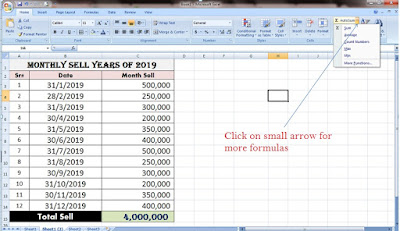
In Microsoft Excel Autosum tab/button use for multipurpose tools. When you want to total a particular row or column you can use this function. When you just click on AutoSum, Excel automatically enters a formula and immediately gives the result. For example, if you want to A1 to A12 sum/total select the range and click on auto sum it automatically insert total on A13 column =SUM(A1:A12).
 |
| how to use autosum in excel 2007 |
When you click on auto sum drop-down small arrow here also you can find other formulas like Average, Count Number, Max, Min.
 |
| Autosum tab more formula |
Average Formula:
To get the average from all the value uses the average function. For example, if a row or column contains 1,2,3… to 12 number, the sum of these number come 78 and when divided by total number than average come 6.5. In this way, the average formula works.
Min Formula:
To find the minimum value from a set of numbers, use the MIN function.
Select the cell where you want the result to appear and click on Min.
Max Formula:
To find the maximum value from a set of numbers, use the MAX function.
Select the cell where you want the result to appear and click on Max.
Count Number:
Count Numbers can be used to find out how many cells contain value/text. Count number formula counts the cell and gives the result. For example, if you put the value/text in larger columns or rows and you want to find how many columns or row contain on data count number formula automatically count row/column and provide results.
 |
| Average,count number,max,min formula |
If you want to get the smallest 3 values apply the formula =SMALL(B2:F10,1)&", "&SMALL(B2:F10,2)&", "&SMALL(B2:F10,3)
If you want to get the largest 3 values apply the formula =LARGE(B2:F10,1)&", "&LARGE(B2:F10,2)&", "&LARGE(B2:F10,3)
What is cell styles and how to apply?
In Microsoft Excel, a cell style contains different formatting options, which you can quickly apply on your worksheet such as font, sizes & color, comma, percentage, currency formats, cell borders, and shading, etc. You can also modify or duplicate a cell style to create your own, custom cell style. Cell styles are based on the document theme that is applied to the whole workbook. Suppose if you apply currency format it only add dollar sign on number/value.
Please see the below image for better understanding.
In Microsoft Excel Insert or Delete is a function that can use inserts/delete row or column in a worksheet. Also, we can add a sheet by using these tab options.
When you click the Insert button, Excel displays the Insert Function dialog box. You can use its options to insert cells/rows or sheet
To insert new cells, rows, or columns in Excel worksheet, follow these steps:
Select the cells, rows, or columns where you want to add the new, blank cells.
Click on Insert button the drop-down arrow in the Cells group of the Home tab.
Click Insert Cells on the drop-down menu and choose the option required for your work.
OR
Shortkey to insert a row to quickly insert a row in Excel, select a row and use the shortcut CTRL SHIFT +
 |
| how to insert a row in excel |
 |
| insert a row in excel |
Another useful option in insert function is you can change row/column up or down and left or right without change the whole data.
 |
| insert shift cell down |
To delete the cell, row, or column in Excel worksheet follow these steps:
Select the cells, rows, or columns you want to delete.
Click on Delete button the drop-down arrow in the Cells group of the Home tab.
Click Delete Cells on the drop-down menu and choose option required for your work.
OR
Short key to delete row to quickly delete a row in Excel, select a row and use the shortcut (control+minious) CTRL -.
 |
| how to delete row |
Note: The screenshots in this blog were taken from Excel 2007. If you have a different version your view might be slightly different, but the functionality is the same.
To be continuous..




good Step for learn and earn for bigginers.
ReplyDeleteThanks for your support and positive feedback
ReplyDeleteThis is very interesting, but it is necessary to click on this link: skills to learn in 2021
ReplyDeleteMS. Sobia may can i help you?
Delete